
How does a spam filter know that an email containing the phrase "Congratulations, you won!" is 99% likely to be junk? How does a recommendation engine guess which product a user is most likely to buy next?
The answer isn't magic—it's Probability.
In Data Science and Machine Learning, we almost never have complete, 100% perfect information about the world. Instead, we deal with uncertainty, noise, and incomplete data. Probability provides the exact language and tools needed to quantify that uncertainty and make smart, automated decisions.
1. Sample Spaces, Events, and Probability Basics
To understand probability, let's start with three simple building blocks:
Sample Space (S): The set of all possible outcomes of a process.
- Example: If you roll a standard 6-sided die, your sample space is S = 1, 2, 3, 4, 5, 6.
- Real-World ML Example: If a user visits your e-commerce site, the sample space for their immediate action might be S = {Buy, Abandon Cart, Keep Browsing}.
Event (E): A specific outcome (or combination of outcomes) you care about. An event is a subset of the sample space.
- Example: Rolling an even number on a die gives the event E = 2, 4, 6.
Probability (P(E)): A number between 0 and 1 that measures how likely event E is to happen.
- P(E) = 0 means the event is impossible.
- P(E) = 1 means the event is guaranteed to happen.
Kolmogorov's 3 Rules of Probability
In 1933, mathematician Andrey Kolmogorov defined three foundational rules that govern all of probability:
- Rule 1 (Non-negativity): Probability can never be negative: P(E) >= 0.
- Rule 2 (Total Certainty): The probability of something in the sample space happening is always 1: P(S) = 1.
- Rule 3 (Additivity): If two events cannot happen at the same time (mutually exclusive), the probability of either happening is the sum of their individual probabilities:
Math Expression
$$P(A or B) = P(A) + P(B)$$
2. Conditional Probability & Bayes' Theorem (The Spam Filter Analogy)
In the real world, events don't happen in isolation. New information updates what we know.
Conditional Probability is the likelihood of event A happening, given that event B has already happened. We write this as P(A|B).
Math Expression
$$P(A|B) = \frac{P(A \cap B)}{P(B)}$$
Real-World Example: Detecting Spam
Suppose we are building a simple email spam filter.
- Event A: The email is Spam.
- Event B: The email contains the word "FREE".
We don't just want to know how many emails are spam overall; we want to know: Given that an incoming email contains the word "FREE", what is the probability that it is Spam?
By turning this conditional logic around, we derive Bayes' Theorem:
Math Expression
$$P(\text{Spam} \vert{} \text{"FREE"}) = \frac{P(\text{"FREE"} \vert{} \text{Spam}) \times P(\text{Spam})}{P(\text{"FREE"})}$$
- P(Spam): The general chance an email is spam (our Prior belief).
- P("FREE" | Spam): How often spam emails use the word "FREE" (the Likelihood).
- P("FREE"): How often the word "FREE" appears across all emails (the Evidence).
- P(Spam | "FREE"): The updated probability after seeing the word "FREE" (our Posterior belief).
3. Random Variables: Translating the World into Numbers
Machine learning algorithms don't work directly with words like "Spam" or "Buy"—they process numbers. A Random Variable (X) is simply a mathematical rule that converts real-world outcomes into numerical values.
There are two main types of random variables:
A. Discrete Random Variables (Countable Values)
These represent whole numbers or distinct categories.
- Examples: The number of customer support tickets received per hour (X = 0, 1, 2, 3, ...), or whether a user clicks an ad (X = 1 for click, X = 0 for no click).
The probability rule for discrete variables is called a Probability Mass Function (PMF). It gives the exact probability for each individual value x:
Math Expression
$$p(x) = P(X = x)$$
B. Continuous Random Variables (Measurable Ranges)
These represent measurements that can take on any real value within a continuous range.
- Examples: The exact time a user spends on a webpage (e.g., 14.352 seconds), or the exact price of a house.
For continuous variables, the probability of hitting an exact single number (like spending exactly 14.00000000... seconds) is effectively zero. Instead, we measure probability over an interval (e.g., spending between 10 and 15 seconds) using a Probability Density Function (PDF), denoted as f(x).
The probability is equal to the area under the PDF curve between two points:
Math Expression
$$P(a \le X \le b) = \int_{a}^{b} f(x) \,dx$$
4. Summarizing Data: Expectation and Variance
When working with thousands of data points, we need a few summary metrics to describe their behavior quickly: Where is the center? and How spread out is the data?
The Expected Value (E[X]): The Center of Mass
The Expected Value (or mean, mu) is the probability-weighted average of all possible outcomes. Think of it as what you would expect to get on average if you ran an experiment thousands of times.
- For Discrete Variables:
Math Expression
$$E[X] = \sum x \cdot p(x)$$
- For Continuous Variables:
Math Expression
$$E[X] = \int_{-\infty}^{\infty} x \cdot f(x) \,dx$$
Example: If a game pays out $10 with a probability of 20% and $0 with a probability of 80%, the expected value is:
Math Expression
$$E[X] = (10 \times 0.20) + (0 \times 0.80) = \$2.00$$
Variance (Var(X)): The Measure of Spread
Variance (sigma2) tells us how far individual data points tend to deviate from the mean. High variance means unpredictable, highly spread-out data; low variance means data points are clustered closely around the average.
The formula for variance is:
Math Expression
$$Var(X) = E[(X - \mu)^2] = E[X^2] - (E[X])^2$$
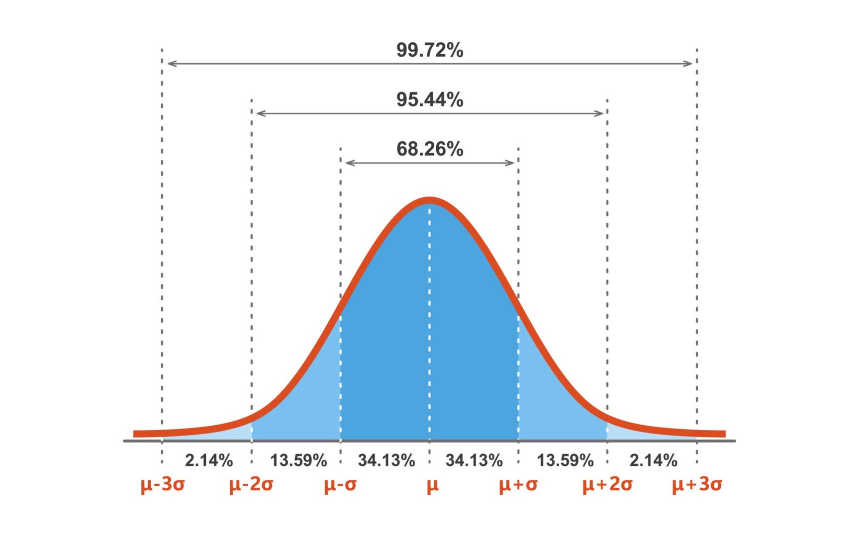
5. The Central Limit Theorem (CLT): Why Bell Curves Rule the World
Imagine taking a survey on household incomes. A few billionaires will heavily skew the results to the right. The raw data is definitely not a symmetric bell curve.
However, if you take 100 random people, compute their average income, and repeat this process 1,000 times, a surprising thing happens: The distribution of those averages will form a neat, symmetric bell curve (Normal Distribution).
This is the Central Limit Theorem (CLT).
The Central Limit Theorem: No matter what shape your raw data starts with (skewed, flat, or discrete), the distribution of the sample averages will always approach a Normal Distribution as your sample size (n) gets larger (typically n >= 30).
This is why the Normal Distribution is so central to data science—it allows us to make reliable statistical predictions about large populations even when the underlying raw data is messy and non-normal.
6. Hands-On Python: Implementing Probability Concepts from Scratch
Let's translate these statistical concepts into pure, readable Python code without relying on complex external libraries.
Python
import random
import math

# ==========================================
# 1. Expected Value and Variance from Scratch
# ==========================================

# Define a discrete random variable (e.g., rolling a biased 6-sided die)
# Values: [1, 2, 3, 4, 5, 6]
outcomes = [1, 2, 3, 4, 5, 6]
probabilities = [0.1, 0.1, 0.1, 0.1, 0.1, 0.5] # Biased towards rolling a 6

def calculate_expected_value(values, probs):
    """Calculates E[X] = sum(x * p(x))"""
    return sum(x * p for x, p in zip(values, probs))

def calculate_variance(values, probs):
    """Calculates Var(X) = E[X^2] - (E[X])^2"""
    expected_x = calculate_expected_value(values, probs)
    expected_x_squared = sum((x ** 2) * p for x, p in zip(values, probs))
    return expected_x_squared - (expected_x ** 2)

mean = calculate_expected_value(outcomes, probabilities)
variance = calculate_variance(outcomes, probabilities)

print(f"Biased Die -> Expected Value E[X]: {mean:.2f}")
print(f"Biased Die -> Variance Var(X): {variance:.2f}")


# ==========================================
# 2. Simulating the Central Limit Theorem
# ==========================================

def get_skewed_sample(size):
    """Generates a highly skewed sample (exponential distribution)."""
    return [random.expovariate(lambd=0.5) for _ in range(size)]

def simulate_central_limit_theorem(sample_size=35, num_experiments=1000):
    """
    Repeatedly calculates the average of random samples
    to demonstrate convergence to a normal distribution.
    """
    sample_means = []

    for _ in range(num_experiments):
        sample = get_skewed_sample(sample_size)
        sample_mean = sum(sample) / len(sample)
        sample_means.append(sample_mean)

    return sample_means

# Run simulation
sample_means = simulate_central_limit_theorem(sample_size=40, num_experiments=10000)

overall_mean = sum(sample_means) / len(sample_means)
print(f"\nCLT Simulation (10,000 experiments):")
print(f"Average of all Sample Means: {overall_mean:.2f} (Expected Population Mean: 2.00)")
Key Takeaways
- Probability is the mathematical foundation for handling uncertainty in AI and ML.
- Bayes' Theorem lets us update our prediction when new evidence arrives.
- Random Variables map real-world outcomes into numbers (Discrete for counts, Continuous for measurements).
- The Central Limit Theorem explains why sample averages follow a bell curve, making large-scale statistical inference possible.


Comments (0)
No comments yet. Be the first to share your thoughts.