Why Statistics Comes Before Machine Learning

Picture someone learning machine learning for the first time. They find a dataset of students, their hours of study, and their exam scores. They load it, call a regression function from a library, and get a result: studying more barely moves the score. The line the model draws is almost flat. They shrug and conclude that studying does not matter much for this exam.

The model was not lying. It did exactly what it was told: find the line that best fits the numbers it was given. The problem was upstream, in the data itself. One row had a typo. A student who studied for 10 hours was recorded as having studied for 100 hours, with the same score as before. That single wrong number was enough to flatten the whole relationship the model was supposed to learn.

Nobody caught this because nobody looked. The data went straight from a file into a model, and the model's output went straight into a conclusion. A few seconds spent on simple statistics, a mean, a maximum, a quick look at the range of values, would have caught the error before it ever reached the model. That gap, between collecting data and understanding it, is exactly what statistics exists to close, and it is why this learning path starts here rather than with a model.

Statistics is the discipline of describing what you have and reasoning carefully about what you do not. It splits naturally into two halves.

Machine learning is neither of these halves by itself. It is a set of techniques for building functions that make predictions from data, usually by minimising some measure of error. But every step of that process, from the data you feed in, to the error measure you minimise, to the number you report at the end, is a statistical object. You can run the algorithms without knowing this. You cannot judge whether the result means anything without it.

Every dataset has errors, missing values, duplicate rows, and points that do not belong. A model has no way of knowing this. It treats every row as equally trustworthy unless you tell it otherwise. The only way to tell it otherwise is to look first, and looking means computing simple summaries: how many rows are there, what is the smallest and largest value in each column, what is a typical value, how much do values vary. These are the first descriptive statistics anyone learns, and they are also the cheapest insurance against the kind of error in the opening example.

Almost every machine learning workflow involves splitting data into a part used to fit the model and a part held back to check it. This split is a sampling decision. If the holdout part is not representative of the data the model will see in the real world, the check is meaningless even if the number it produces looks precise. Understanding what makes a sample representative, and what makes it biased, is a statistics question, not a modelling question, and it is covered later in this path under sampling and sampling bias.

Many models carry quiet assumptions about the data. A plain linear regression assumes the relationship between input and output is roughly a straight line and that the scatter around that line is fairly even. Some methods behave better when the data roughly follows a particular distribution, or struggle when one variable has a much wider spread than another. None of these assumptions are visible in the code that fits the model. They become visible when you plot the data, look at its shape, and check its spread, which is exactly what descriptive statistics teaches you to do before you trust a result.

The single number a model reports at the end, an accuracy, an error rate, an average difference between predicted and actual values, is itself a statistic. A mean error of 2 points on an exam score sounds small until you learn that most errors are near zero but a few are enormous, which a mean alone will hide. Reporting one number without also reporting how spread out the errors are, or how unusual the extreme cases are, is a common way that a model's real performance gets overstated. Spotting this requires the same tools used to describe any other dataset: centre, spread, shape.

Go back to the ten students from the opening scenario and look at the actual numbers. Here is the original, correct data: hours studied and exam score for each student.

The pattern is clear just from reading the list: as hours go up, scores go up in a fairly steady way. A model fit to this data would find a line with a positive slope, meaning each extra hour of study is associated with a higher score.

Now suppose the last row has a data entry error. Someone meant to type 10 hours but typed 100, and the score stays 85, because the score itself was recorded correctly from a separate system. The dataset now reads 1, 2, 3, 4, 5, 6, 7, 8, 9, 100 for hours, with the same scores as before.

Look at what happens to a basic descriptive statistic, the mean, before and after this single change. The mean of the original hours is the sum of all ten values divided by ten: 1 + 2 + 3 + 4 + 5 + 6 + 7 + 8 + 9 + 10 equals 55, and 55 divided by 10 is 5.5. That is a believable typical value for hours studied before an exam. After the typo, the sum becomes 1 + 2 + 3 + 4 + 5 + 6 + 7 + 8 + 9 + 100, which is 145, and 145 divided by 10 is 14.5. A single wrong entry nearly tripled the average. If the realistic range for this assignment was, say, zero to twenty hours, a mean of 14.5 pulled almost entirely by one value of 100 should immediately look suspicious to anyone who stops to compute it.

This is also exactly what breaks the model. A line fit to predict score from hours tries to find the slope and starting point that minimise the overall error across all ten points. With the typo in place, one point sits far to the right of all the others on the hours axis, at 100, while its score, 85, is only slightly higher than the next highest score. To keep the error at that one distant point from being enormous, the fitting process is forced to flatten the line, which drags down the slope for every other, correctly recorded student too. The model's conclusion, that studying barely matters, is an artefact of one bad number, not a fact about the students.

A short piece of code makes the check concrete. It does not need a machine learning library, just two basic descriptive statistics: the mean and the maximum.

hours = [1, 2, 3, 4, 5, 6, 7, 8, 9, 100]

mean_hours = sum(hours) / len(hours)
max_hours = max(hours)

print("mean hours:", mean_hours)
print("max hours:", max_hours)

Running this (plain Python, no external libraries needed) prints a mean of 14.5 and a maximum of 100. Neither number fits what is plausible for hours spent studying for one exam. That mismatch, about eleven times larger than the next largest value and a mean far above what the bulk of the data suggests, is the kind of signal descriptive statistics is built to surface. Catching it takes seconds and happens before any model is trained. Catching the same problem by only looking at model output, if you catch it at all, takes much longer and requires already suspecting something is wrong.

None of this required inferential statistics, hypothesis tests, or anything advanced. It required computing a mean and a maximum and comparing them to what a sensible value should look like. That is the entire argument for putting statistics first: the tools that catch this kind of error are simple, but they are only useful if you reach for them before, not after, you trust a result.

The typo example is one specific failure. In practice, skipping statistics tends to produce the same handful of mistakes over and over, across very different datasets and problems.

ice cream

sales and drownings both rise in hot weather, without either one causing the other.

Every one of these mistakes is avoidable, and every one of them is avoided the same way: by treating the data itself as something to understand before it becomes something to model.

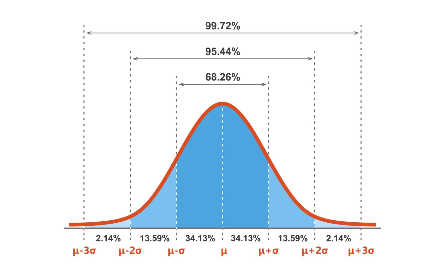
This series works through the statistics that come up constantly in data work, in the order they tend to be needed, using small datasets you can check by hand. It starts with the kinds of data you will encounter, because the right summary for a category is not the right summary for a measurement. It then builds the three ways of describing a typical value, the several ways of describing spread, and the tools for seeing a distribution's shape, including the normal distribution and the rule of thumb that goes with it. From there it covers how to find and reason about outliers, how to measure whether two variables move together and where that measure misleads, and how samples differ from the full populations they are drawn from. The path closes with two hands-on pieces: describing a real dataset using the pandas library, and a full statistical profile of a city's housing prices, where everything from the earlier articles gets used together on one dataset.

None of this is a detour before the real work of machine learning. It is the real work, done at the stage where it is cheapest to fix a mistake: before a model has been trained, before a dashboard has been built, before a decision has been made on the strength of a number nobody checked.

Machine learning produces an answer whether or not the data behind it makes sense. Statistics is how you find out whether it should. The worked example here showed how a single incorrect value in a tiny dataset was enough to flatten a model's conclusion, and how two of the simplest statistics available, a mean and a maximum, were enough to catch it before any model was trained. The rest of this path builds outward from that same habit: describe the data carefully, understand its centre, its spread, and its shape, before asking a model to learn from it.

The next article looks at the different kinds of data you will meet, categorical, ordinal, discrete and continuous, and why the type of data you have determines which summaries and charts are even valid to use on it.